Understanding Data Cubes
One reason that radio astronomy has a harder time of it is that we generally make 3D "data cubes" rather than normal 2D images. This is by necessity. The exact frequency or wavelength of HI (atomic hydrogen) emission depends on exactly how fast it's moving towards or away from us. If it's not moving at all it emits at about 21.1 cm; moving away from us it emits at longer wavelengths (lower frequencies) and vice-versa if moving towards us. We often refer to all of it as 21 cm emission by convention, regardless of its exact wavelength*, which is okay since the change due to velocity is usually quite small.
* Astronomers can be oddly pedantic yet perversely liberal. Sometimes we don't care as long as a value is correct to within a factor of ten, but woe betide anyone who misuses a term.
To detect a galaxy, we must tune our receivers very precisely to the correct frequency, depending on how far away the galaxy is (i.e. how fast it's moving along our line of sight – for the details of this, and the reasons we make different estimates of velocities, go here) and how fast it's rotating. For this we need receivers that are sensitive to many thousands of different frequency channels at all once, which, fortunately, we can build ! So with a radio telescope we don't just make one image of the sky wherever we point, but thousands, each corresponding to a slightly different velocity.
Manipulating these data cubes becomes much easier if we abandon any boring pretence that each axis must corresponds to position in space. Instead, we simply use velocity to stand in for distance, and then we very easily assemble the data into a truly 3D structure. This enables us to visualise the entire thing all at once, rather than insisting on going through it channel by channel – a procedure which is so dull it's just not funny. (For a couple more videos showing how this data can be shown in 3D, see this and then this)
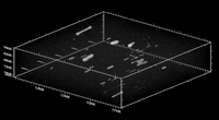
Using velocity as the third axis causes some strange effects. On the large scale, thanks to Hubble's Law we know that velocity and distance are directly equivalent, except for very localised effects. This means that in the images above, the centre of each "line" (blob) corresponds to the systemic velocity of each galaxy, i.e. its distance. For these low-resolution cubes the situation is easy enough to interpret : velocity of blob = distance of galaxy; width of blob = rotation speed of galaxy; brightness of blob (at any given distance) = mass of gas.
But why do they look like blobs anyway ? Well, when we have a galaxy that's close enough, and/or a telescope with high enough spatial resolution, they don't. On the very small scales of individual galaxies themselves, velocity is dependent on how fast the galaxy rotates, which has nothing at all to do with distance ! If a galaxy is close enough, and/or our survey has enough resolution, galaxies in our radio* data cubes look like this :
* It's hard to do this at the much shorter optical wavelengths, but it is possible, and has become much more common in recent years.
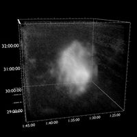
Here one has to abandon any idea that the third axis has any resemblance to distance. The reason that such galaxies look like blobs in the lower resolution data is that spatial resolution is not linked to velocity resolution. Suppose we move this same galaxy further and further away. Then on the sky, it will appear smaller and smaller and less and less detailed. But this is no way affects the accuracy with which we can measure the frequency of the emission : the image gets spatially blurrier, but the kinematic resolution remains just as sharp.
A word about spectra
Most HI detections are unresolved blobs. The 3D view is very nice (and useful !) for understanding the full structure of the data set, but we don't really need this – most of the time – for analysing the data. In fact we can reduce it down to a single dimension, a spectrum. At any point in our data cube we can plot the brightness of the emission as a function of frequency (velocity). Mostly this is just noise, but the galaxies stand out as much brighter regions.
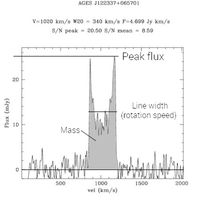
As mentioned, the different components provide us with quite a lot of information : distance (from the average velocity, which is about 1000 km/s in the above example), rotation speed, HI mass. The shape of the spectrum itself can also be useful, for example if it's very lop-sided the galaxy might have been disturbed; the double-horn shape* tells us that most of the gas is moving at a single velocity (equivalent to the notorious flat rotation curves). Combine all this with optical data and the number of parameters we can measure increases substantially.
* This paper gives a nice overview of the different profile shapes, as well as presenting a way of measuring them.
Spectra by themselves don't tell us everything though. We need to look at the 3D set in its entirety because not all HI is associated with optically bright galaxies : we can't just point the radio telescope at all the known galaxies and hope to find all the gas. And some galaxies have extended HI features (tails, bridges, streams and other oddities) which are resolved, and need to be looked at as ordinary 2D images. Still, most of the time, spectra are where it's at.